摘要: 视觉变换器(ViTs)在各种计算机视觉应用中已经达到了最先进的性能。然而,这些模型具有相当的存储和计算开销,这使得它们在边缘设备上的部署和高效推理变得具有挑战性。量化是一种减少模型复杂度的有前景的方法,而二进制算术管道可以使量化模型执行高效的仅整数推理。不幸的是,二进制算法基于卷积神经网络中的均匀性条件,这不适用于ViTs中的非线性组件,使得ViTs的仅整数推理成为一个开放问题。在本文中,我们提出了I-ViT,一种ViTs的仅整数量化方案,以使ViTs能够使用整数算术和位移来执行整个推理的计算图,而无需任何浮点算术。在I-ViT中,线性操作(例如,MatMul和Dense)遵循带有二进制算术的仅整数管道,非线性操作(例如,Softmax,GELU和LayerNorm)通过所提出的轻量级仅整数算术方法进行近似。更具体地说,I-ViT应用了所提出的Shiftmax和ShiftGELU,这些方法设计为使用整数位移来近似相应的浮点操作。我们在各种基准模型上评估了I-ViT,结果显示仅整数INT8量化的准确性与全精度(FP)基线相当(甚至略高)。此外,我们利用TVM在GPU的整数算术单元上进行实际硬件部署,与FP模型相比,实现了3.72∼4.11×的推理加速。Pytorch和TVM的代码已在https://github.com/zkkli/I-ViT 上发布。
1. Intro
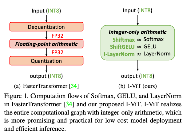
传统的CNN相关的量化工作中一般要求被量化的操作具有“齐次性”,只适合线性或者分段线性的操作。但是ViT中的GELU,Softmax等操作都不是线性的。对比的FastTransformer直接保留了中间的FP32操作(防止掉点),代价是推理非常慢,因为推理速度完全受制于浮点运算单元等,而它们的性能显然不如纯整型的计算过程。
Contribution:
“the first work on integer-only quantization for ViTs”
novel light-weight integer approximations for non-linear operations, in particular, Shiftmax and ShiftGELU use integer bit- shifting to accomplish most arithmetic, which fully benefit from the efficient hardware logic.
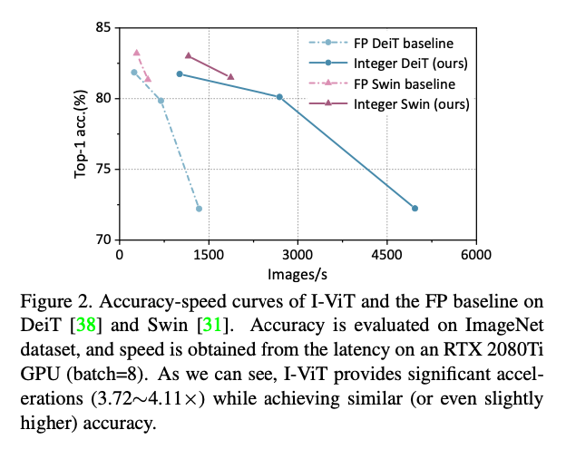
evaluated on various models for the large-scale classification task, achieving compression with similar (or even slightly higher) accuracy. Moreover, we de- ploy I-ViT on an RTX 2080Ti GPU using TVM, which accelerates the integer-only inference of ViTs with Turing Tensor Cores, achieving a 3.72∼4.11× speedup over the FP model
ViT, DeiT, 总体来讲在大数据集上超过了传统的基于卷积的神经网络,但是参数量很大,计算的overhead很高。
2.2. Model Quantization
之前的量化工作集中在CNN上,比如DoReFa,LQ-NET,LSQ,但是在ViT上没用。
ViT上的量化工作有Q-ViT,PTQ4ViT,FQ-ViT,RepQ-ViT。但是上面这些量化的工作在inference的过程中还是需要有浮点的介入(Quantization & dequantization的过程),效率不高。
2.3. Integer-only quantization
相比有浮点介入的操作,纯整型的pipeline效率肯定更高一些。I-BERT在BERT上实现了纯整型的推理,但是中间的高阶多项式推理的开销比较大,并且两者使用的数据不同,分布不同,I-BERT中的估计不一定准确。在这篇文章之前还没有在ViT上实现的纯整形量化。
3. Methodology
3.1. Overview
Formula:
Multi-head Self-Attention:
X ^ = MSA ( LayerNorm ( X ) ) + X \hat{X}=\text{MSA}(\text{LayerNorm}(X))+X X ^ = MSA ( LayerNorm ( X )) + X
Multi-Layer Perceptron:
Y = MLP ( LayerNorm ( X ^ ) ) + X ^ Y=\text{MLP}(\text{LayerNorm}(\hat{X}))+\hat{X} Y = MLP ( LayerNorm ( X ^ )) + X ^
MSA ( X ) = Concat ( Attn 1 , Attn 2 , … , Attn n ) W O where Attn i = Softmax ( Q i ⋅ K i T d ) V i \text{MSA}(X) = \text{Concat}(\text{Attn}_1, \text{Attn}_2, \dots, \text{Attn}_n) W^O\\\text{where } \text{Attn}_i = \text{Softmax} \left( \frac{Q_i \cdot K_i^T}{\sqrt{d}} \right) V_i MSA ( X ) = Concat ( Attn 1 , Attn 2 , … , Attn n ) W O where Attn i = Softmax ( d Q i ⋅ K i T ) V i
MLP ( X ^ ) = GELU ( X ^ W 1 + b 1 ) W 2 + b 2 . \text{MLP}(\hat{X}) = \text{GELU}(\hat{X}W_1 + b_1)W_2 + b_2. MLP ( X ^ ) = GELU ( X ^ W 1 + b 1 ) W 2 + b 2 .
量化是均匀对称量化:
I = ⌊ clip ( R , − m , m ) S ⌉ , where S = 2 m 2 k − 1 I = \left\lfloor \frac{\text{clip}(R, -m, m)}{S} \right\rceil, \quad \text{where } S = \frac{2m}{2^k - 1} I = ⌊ S clip ( R , − m , m ) ⌉ , where S = 2 k − 1 2 m
上面量化的操作只适合线性的操作而不适合softmax等非线性的操作,因此文章中提出了一些型的方法逼近原本的非线性操作,并且利用移位等操作减小开销。
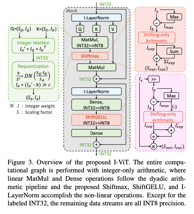
3.2. Dyadic Arithmetic for Linear Operations
输入要包括S S S 和I I I 两个参数,比如输入Q = ( S Q , I Q ) Q=(S_Q, I_Q) Q = ( S Q , I Q ) 和K = ( S K , I K ) K=(S_K, I_K) K = ( S K , I K ) ,矩阵乘的过程写作:
A ′ = S A ⋅ I A = S Q ⋅ S K ⋅ ( I Q ∗ I K T ) A' = S_A \cdot I_A = S_Q \cdot S_K \cdot (I_Q \ast I_K^T) A ′ = S A ⋅ I A = S Q ⋅ S K ⋅ ( I Q ∗ I K T )
然后要把I A ′ I'_A I A ′ reduce到INT8上来:
I A = ⌊ S A ′ ⋅ I A ′ S A ⌉ = ⌊ S Q ⋅ S K S A ⋅ ( I Q ∗ I K T ) ⌉ I_A = \left\lfloor \frac{S_A' \cdot I_A'}{S_A} \right\rceil = \left\lfloor \frac{S_Q \cdot S_K }{S_A} \cdot (I_Q \ast I_K^T)\right \rceil I A = ⌊ S A S A ′ ⋅ I A ′ ⌉ = ⌊ S A S Q ⋅ S K ⋅ ( I Q ∗ I K T ) ⌉
缩放因子S都是浮点数,但是一般重新scale到
DN ( S q ⋅ S K S A ) = b 2 c \text{DN}\left (\frac{S_q \cdot S_K}{S_A}\right )=\frac{b}{2^c} DN ( S A S q ⋅ S K ) = 2 c b
所以最终有:
I A = ( b ⋅ ( I Q ∗ I K T ) ) ≫ c I_A = (b \cdot (I_Q \ast I_K^T)) \gg c I A = ( b ⋅ ( I Q ∗ I K T )) ≫ c
这个操作过程中就不涉及任何浮点数,只有纯整型的操作了。
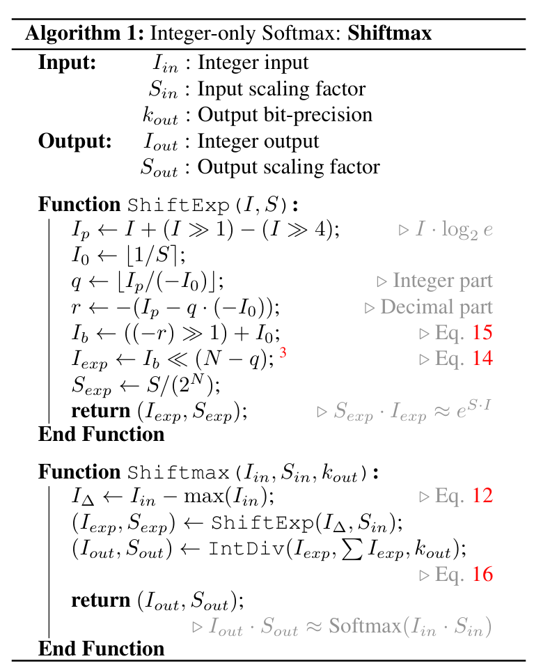
3.3. Integer-only Softmax: Shiftmax
普通softmax:
Softmax ( x i ) = e x i ∑ j e x j = e S x i ⋅ I x i ∑ j e S x j ⋅ I x j \text{Softmax}(x_i) = \frac{e^{x_i}}{\sum_j e^{x_j}} = \frac{e^{S_{x_i} \cdot I_{x_i}}}{\sum_j e^{S_{x_j} \cdot I_{x_j}}} Softmax ( x i ) = ∑ j e x j e x i = ∑ j e S x j ⋅ I x j e S x i ⋅ I x i
文章里做改进的实际上也是减去max之后的safe-softmax:
Softmax ( x i ) = e S Δ i ⋅ I Δ i ∑ j e S Δ j ⋅ I Δ j = e S x i ⋅ ( I x i − I max ) ∑ j e S x j ⋅ ( I x j − I max ) \text{Softmax}(x_i) = \frac{e^{S_{\Delta_i} \cdot I_{\Delta_i}}}{\sum_j e^{S_{\Delta_j} \cdot I_{\Delta_j}}} = \frac{e^{S_{x_i} \cdot (I_{x_i} - I_{\text{max}})}}{\sum_j e^{S_{x_j} \cdot (I_{x_j} - I_{\text{max}})}} Softmax ( x i ) = ∑ j e S Δ j ⋅ I Δ j e S Δ i ⋅ I Δ i = ∑ j e S x j ⋅ ( I x j − I max ) e S x i ⋅ ( I x i − I max )
近似:
e S Δ ⋅ I Δ = 2 S Δ ⋅ ( I Δ ⋅ log 2 e ) ≈ 2 S Δ ⋅ ( I Δ + ( I Δ ≫ 1 ) − ( I Δ ≫ 4 ) ) e^{S_\Delta \cdot I_\Delta} = 2^{S_\Delta \cdot (I_\Delta \cdot \log_2 e)} \approx 2^{S_\Delta \cdot (I_\Delta + (I_\Delta \gg 1) - (I_\Delta \gg 4))} e S Δ ⋅ I Δ = 2 S Δ ⋅ ( I Δ ⋅ l o g 2 e ) ≈ 2 S Δ ⋅ ( I Δ + ( I Δ ≫ 1 ) − ( I Δ ≫ 4 ))
2 S Δ ⋅ I p = 2 ( 2 − q ) + S Δ ⋅ ( − r ) = 2 S Δ ⋅ ( − r ) ≫ q 2^{S_\Delta \cdot I_p} = 2^{(2-q) + S_\Delta \cdot (-r)} = 2^{S_\Delta \cdot (-r)} \gg q 2 S Δ ⋅ I p = 2 ( 2 − q ) + S Δ ⋅ ( − r ) = 2 S Δ ⋅ ( − r ) ≫ q
2 S Δ ⋅ I p ≈ [ S Δ ⋅ ( − r ) ] / 2 + 1 = S Δ ⋅ [ ( ( − r ) ≫ 1 ) + I 0 ] 2^{S_\Delta\cdot I_p}\approx [S_\Delta\cdot(-r)]/2+1=S_\Delta\cdot[((-r)\gg1)+I_0] 2 S Δ ⋅ I p ≈ [ S Δ ⋅ ( − r )] /2 + 1 = S Δ ⋅ [(( − r ) ≫ 1 ) + I 0 ]
最终有:
I out i = S A ⋅ I exp i S A ⋅ ∑ j d I exp j = IntDiv ( I exp i , ∑ j d I exp j , k out ) = ( ⌊ 2 M ∑ j I exp j ⌋ ⋅ I exp i ) ≫ ( M − ( k out − 1 ) ) S out i = 1 2 k out − 1 \begin{align*}I_{\text{out}_i} &= \frac{S_A \cdot I_{\text{exp}_i}}{S_A \cdot \sum^d_j I_{\text{exp}_j}} \\&= \text{IntDiv}(I_{\text{exp}_i}, \sum_j^d I_{\text{exp}_j}, k_{\text{out}}) \\&= \left(\left\lfloor \frac{2^M}{\sum_j I_{\text{exp}_j}}\right\rfloor \cdot I_{\text{exp}_i}\right) \gg (M - (k_{\text{out}} - 1)) \\S_{\text{out}_i} &= \frac{1}{2^{k_{\text{out}}-1}}\end{align*} I out i S out i = S A ⋅ ∑ j d I exp j S A ⋅ I exp i = IntDiv ( I exp i , j ∑ d I exp j , k out ) = ( ⌊ ∑ j I exp j 2 M ⌋ ⋅ I exp i ) ≫ ( M − ( k out − 1 )) = 2 k out − 1 1
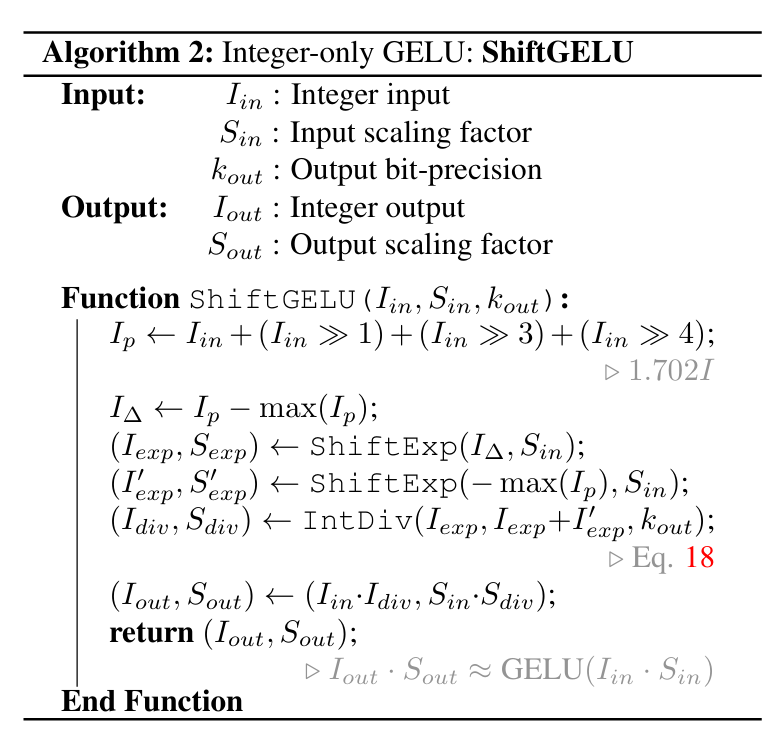
3.4. Integer-only GELU: ShiftGELU
GELU ( x ) = x ⋅ 1 2 π ∫ − ∞ x e − t 2 / 2 d t ≈ x ⋅ σ ( 1.702 x ) = S x ⋅ I x ⋅ σ ( S x ⋅ 1.702 I x ) \text{GELU}(x) = x \cdot \frac{1}{\sqrt{2\pi}} \int_{-\infty}^x e^{-t^2/2} \, dt \\\approx x \cdot \sigma(1.702x) \\= S_x \cdot I_x \cdot \sigma(S_x \cdot 1.702I_x) GELU ( x ) = x ⋅ 2 π 1 ∫ − ∞ x e − t 2 /2 d t ≈ x ⋅ σ ( 1.702 x ) = S x ⋅ I x ⋅ σ ( S x ⋅ 1.702 I x )
1.702 ≈ ( 1.1011 ) b 1.702\approx (1.1011)_b 1.702 ≈ ( 1.1011 ) b ,所以1.702 I x = I x + ( I x ≫ 1 ) + ( I x ≫ 3 ) + ( I x ≫ 4 ) 1.702I_x=I_x+(I_x\gg1)+(I_x\gg3)+(I_x\gg4) 1.702 I x = I x + ( I x ≫ 1 ) + ( I x ≫ 3 ) + ( I x ≫ 4 )
σ ( S x ⋅ I p ) = 1 1 + e − S x ⋅ I p = e S x ⋅ I p e S x ⋅ I p + 1 = e S x ⋅ ( I p − I max ) e S x ⋅ ( I p − I max ) + e S x ⋅ ( − I max ) \sigma(S_x \cdot I_p) = \frac{1}{1 + e^{-S_x \cdot I_p}} = \frac{e^{S_x \cdot I_p}}{e^{S_x \cdot I_p} + 1} = \frac{e^{S_x \cdot (I_p - I_{\text{max}})}}{e^{S_x \cdot (I_p - I_{\text{max}})} + e^{S_x \cdot (-I_{\text{max}})}} σ ( S x ⋅ I p ) = 1 + e − S x ⋅ I p 1 = e S x ⋅ I p + 1 e S x ⋅ I p = e S x ⋅ ( I p − I max ) + e S x ⋅ ( − I max ) e S x ⋅ ( I p − I max )
用Shiftmax里面的估计:
3.5. Integer-only LayerNorm: I-LayerNorm
LayerNorm ( x ) = x − Mean ( x ) Var ( x ) ⋅ γ + β \text{LayerNorm}(x) = \frac{x - \text{Mean}(x)}{\sqrt{\text{Var}(x)}} \cdot \gamma + \beta LayerNorm ( x ) = Var ( x ) x − Mean ( x ) ⋅ γ + β
纯整数算均值和方差都可以,但是开方不行,所以用下面这种迭代的方法估计:
I i + 1 = ( I i + ⌊ Var ( I x ) / I i ⌋ ) / 2 = ( I i + ⌊ Var ( x ) / I i ⌋ ) ≫ 1 I_{i+1} = \left( I_i + \left\lfloor\text{Var}(I_x)/I_i \right\rfloor\right) / 2 \\= \left( I_i + \left\lfloor \text{Var}(x)/I_i \right\rfloor \right) \gg 1 I i + 1 = ( I i + ⌊ Var ( I x ) / I i ⌋ ) /2 = ( I i + ⌊ Var ( x ) / I i ⌋ ) ≫ 1
其中I 0 I_0 I 0 的初始值是2 ⌊ bit ( Var ( I x ) ) / 2 ⌋ 2^{\left\lfloor\text{bit}(\text{Var}(I_x))/2\right\rfloor} 2 ⌊ bit ( Var ( I x )) /2 ⌋ 。最开始设计的收敛判定是I i + 1 ≥ I i I_{i+1}\ge I_i I i + 1 ≥ I i ,但是latency可能会受影响。后面改成固定的10次迭代,大部分情况下都能收敛。
4. Experiments
We evaluate I-ViT in both accuracy on the large-scale classification task and latency on the practical hardware to fully demonstrate the superiority, and I-ViT can accelerate 3.72 ∼ 4.11 × 3.72∼4.11\times 3.72 ∼ 4.11 × over the FP model while achieving similar (or even slightly higher) accuracy.
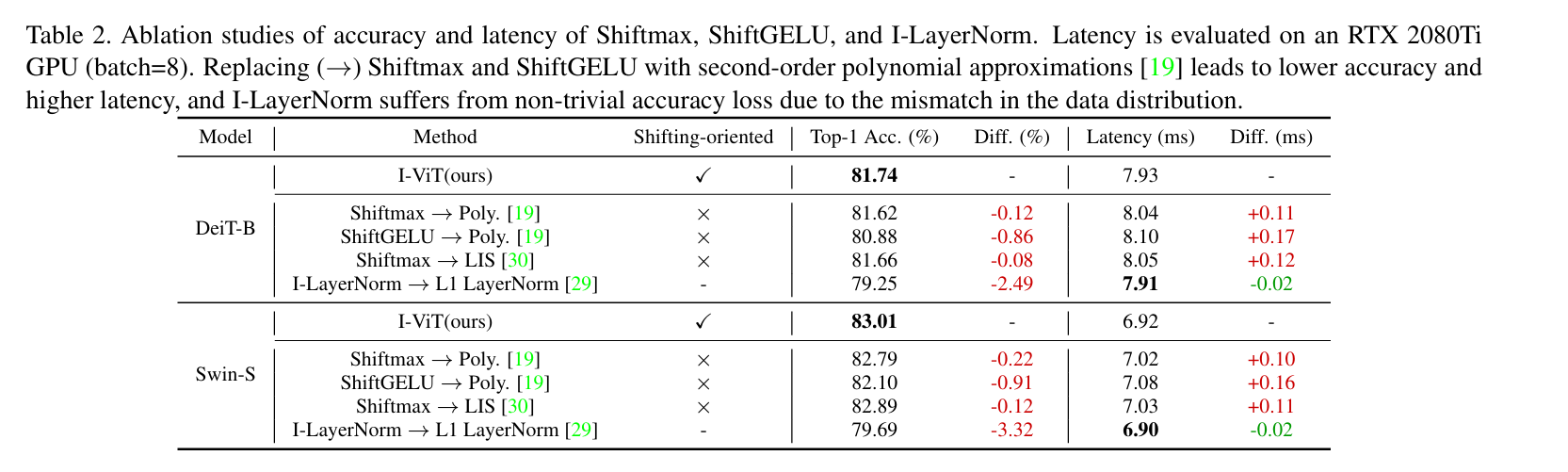
跟FP,FasterTransformer,I-BERT对比,做了L1 LayerNorm in Fully-8bit和Log-Int-Softmax的消融实验。
4.1. Accuracy Evaluation
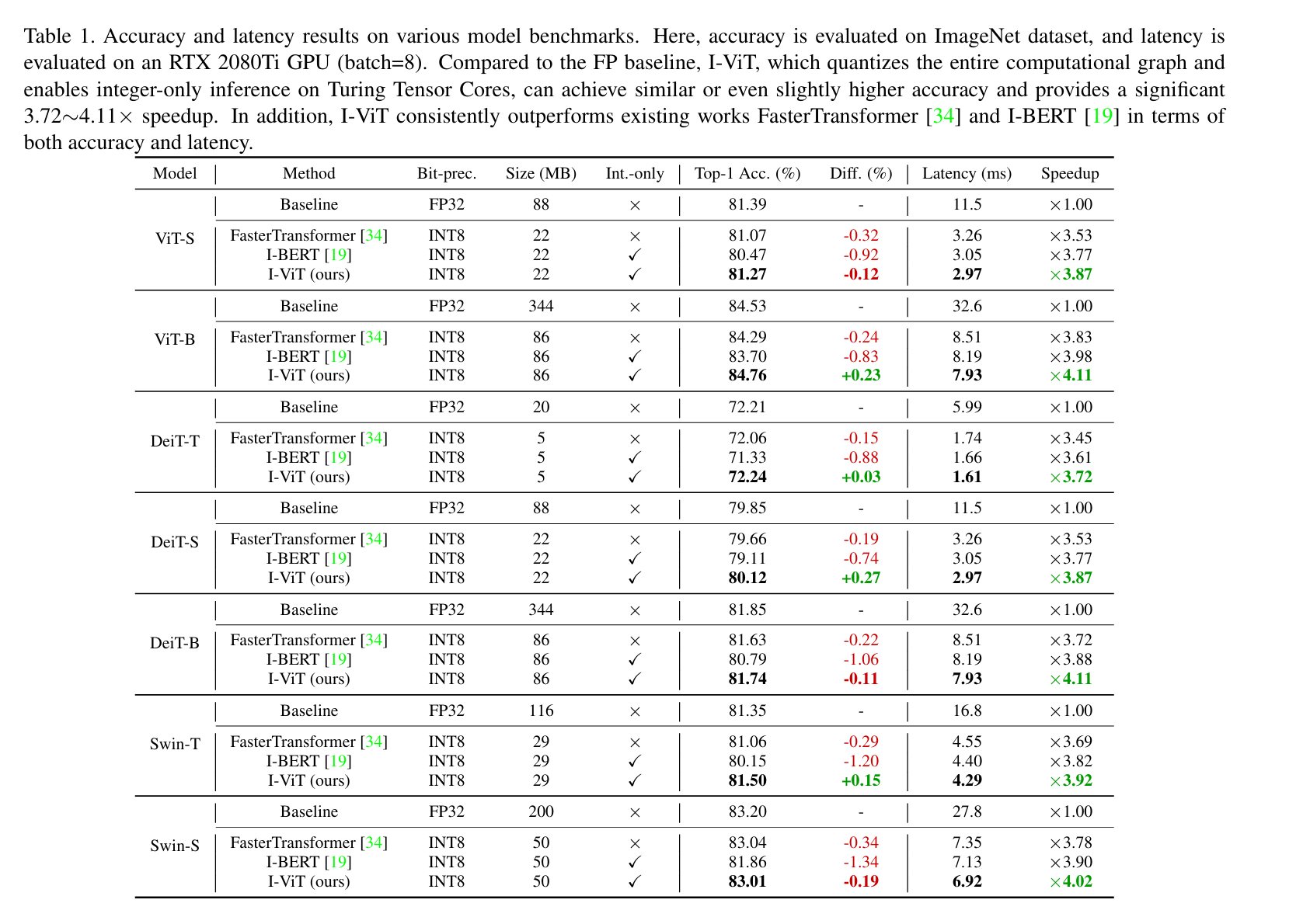
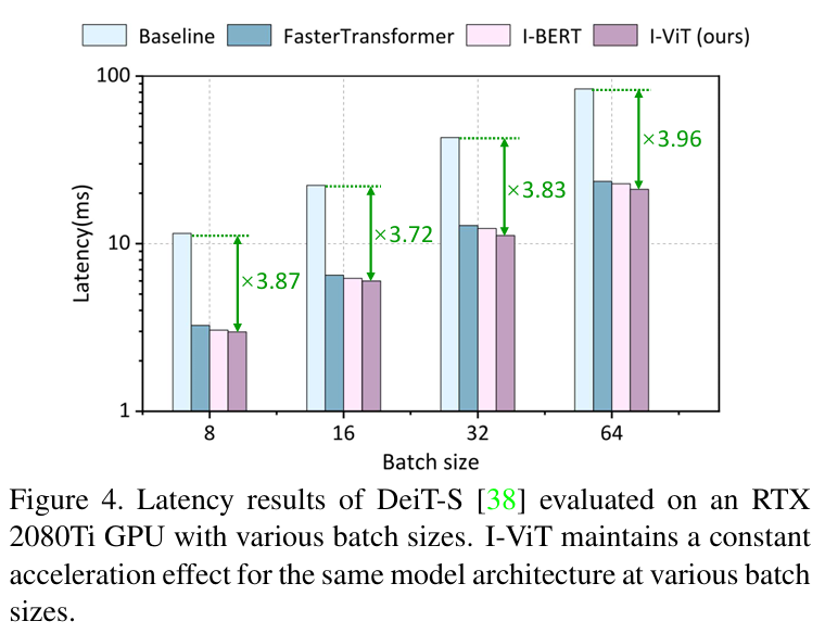
4.2. Latency Evaluation
总体latency的提升大概三到四倍,见下图。好像只比I-BERT强零点几ms。
4.3. Ablation Studies
5. Conclusion
In the future, we will consider deploying I-ViT on dedicated integer-only hardware (e.g., FPGAs) to obtain better acceleration performance. Furthermore, we also plan to extend I-ViT to more complex vision tasks (e.g., object detection and semantic segmentation).